MCMC notes (1)

Recently I was reading articles and books about MCMC, and realized that many materials were not taught in my graduate study. To this end, I decide to make a summary of such content, to assist readers and myself to gain deeper understanding of MCMC in the future. I hope to make this topic a series, although I cannot guarantee its completion. This article is the first one in this hypothetical series, and we are going to introduce an important concept, the geometric ergodicity.

MCMC is an extremely broad topic, so we start with a classical algorithm, the Gibbs sampler. Our target is to sample from a joint distribution $p(x,y)$, which however may have a complicated form. As a result, it is typically hard to directly obtain samples from $p(x,y)$, but in many cases the two conditional distributions, $p(x|y)$ and $p(y|x)$, have simpler forms and exact samplers. This is where the Gibbs sampler can help. Starting with an arbitrary initial value $X_0$, the Gibbs sampler proceeds with the following iterations:

Sample $Y_i\sim p(y|x=X_i)$
Sample $X_{i+1}\sim p(x|y=Y_i)$

Then under some conditions, the distribution of $(X_i,Y_i)$ will converge to $p(x,y)$ as $i$ increases.

To visually demonstrate this process, we use the example in this document. First define the following joint distribution:

$$p(x,y)=\frac{\Gamma(a+b)}{\Gamma(a)\Gamma(b)}\binom{n}{x}y^{x+a-1}(1-y)^{n-x+b-1}.$$

Yes, I know it looks horrible, but with some calculations we can show that

$$X|\{Y=y\}\sim Binomial(n,y),\quad Y|\{X=x\}\sim Beta(a+x,b+n-x).$$

In other words, both conditional distributions are familiar. Using the Gibbs sampler, we construct the following iterations:

Sample $Y_i\sim Beta(a+X_i,b+n-X_i)$
Sample $X_{i+1}\sim Binomial(n,Y_i)$

Fix $a=2,b=5,n=30$, and then we obtain the $X$ samples under different $i$.

n = 30
a = 2
b = 5

sample_y = function(x, a, b, n)  rbeta(length(x), a + x, b + n - x)
sample_x = function(y, a, b, n)  rbinom(length(y), size = n, prob = y)
gibbs = function(x0, niter, a, b, n)
{
    x = x0
    for(i in 1:niter)
    {
        y = sample_y(x, a, b, n)
        x = sample_x(y, a, b, n)
    }
    list(x = x, y = y)
}

set.seed(123)
x0 = rbinom(10000, size = n, prob = 0.5)
res1 = gibbs(x0, niter = 1, a = a, b = b, n = n)
res10 = gibbs(x0, niter = 10, a = a, b = b, n = n)
res100 = gibbs(x0, niter = 100, a = a, b = b, n = n)

In order to study the performance of the Gibbs sampler, we use the obtained samples to approximate the density function of $X$ in a specific iteration, and then compare it with the true density. Below shows the result under $i=1$, $i=10$, and $i=100$:

library(ggplot2)
pmf_x = function(x, a, b, n)
{
    freq_x = table(x)
    est_pmf = numeric(n + 1)
    names(est_pmf) = as.character(0:n)
    est_pmf[names(freq_x)] = freq_x / sum(freq_x)

    ind = 0:n
    true_pmf = choose(n, ind) * beta(a + ind, b + n - ind) / beta(a, b)
    list(ind = ind, true = true_pmf, est = est_pmf)
}
vis_x = function(res, a, b, n)
{
    pmf = pmf_x(res$x, a, b, n)
    gdat = data.frame(ind = rep(pmf$ind, 2), den = c(pmf$est, pmf$true),
                      type = rep(c("Gibbs", "True"), each = n + 1))
    ggplot(gdat, aes(x = ind, y = den, fill = type)) +
        geom_bar(stat = "identity", position = "dodge", alpha = 0.5) +
        scale_fill_brewer("Type", type = "qual", palette = "Set1") +
        xlab("x") + ylab("Density") +
        theme_bw()
}

vis_x(res1, a, b, n)
vis_x(res10, a, b, n)
vis_x(res100, a, b, n)

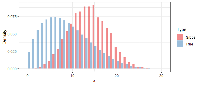
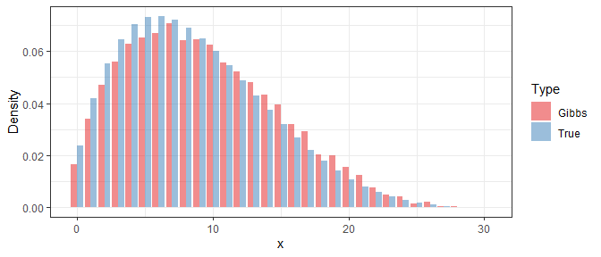
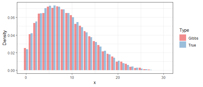
Clearly, even if the Gibbs samples at the beginning are far away from the true distribution, their difference is significantly reduced after 10 iterations. At last, with 100 iterations, the difference is almost invisible.

So here comes one core question in MCMC that is remarkably important yet hard to answer: how many steps of iterations are sufficient?.

To answer this question, we need to first define a metric to evaluate the difference between two distributions. In the example above, the domain of $X$ is $0,1,\ldots,n$. Let $p(x)$ denote the true density function, and $q^{(k)}(x)$ the density of Gibbs samples after $k$ iterations. Then we compute

$$d_{TV}(p,q^{(k)})=\frac{1}{2}\sum_{x=0}^n\vert p(x)-q^{(k)}(x)\vert,$$

which is known as the total variation (TV) distance. We slightly modify our previous code, and record the value of $d_{TV}(p,q^{(k)})$ after each iteration.

dtv = function(x, a, b, n)
{
    pmf = pmf_x(x, a, b, n)
    0.5 * sum(abs(pmf$est - pmf$true))
}
gibbs_dtv = function(x0, niter, a, b, n)
{
    tv = c()
    x = x0
    for(i in 1:niter)
    {
        y = sample_y(x, a, b, n)
        x = sample_x(y, a, b, n)
        tv = c(tv, dtv(x, a, b, n))
    }
    tv
}
set.seed(123)
x0 = rbinom(10000, size = n, prob = 0.5)
tv = gibbs_dtv(x0, niter = 100, a = a, b = b, n = n)
qplot(1:100, tv, geom = c("point", "line")) +
    xlab("# Gibbs Steps") + ylab("TV Distance") + theme_bw()
qplot(1:100, log10(tv), geom = c("point", "line")) +
    xlab("# Gibbs Steps") + ylab("log(TV Distance)") + theme_bw()

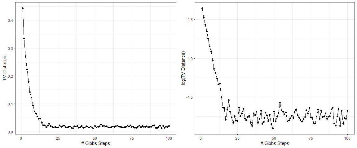
The plot on the left shows the evolution of $d_{TV}(p,q^{(k)})$ with $k$, and the plot on the right illustrates the logarithm of $d_{TV}(p,q^{(k)})$. Interestingly, the dots in the second plot roughly form a straight line in the early stage, which indicates that the TV distance between Gibbs samples and the true density almost decays exponentially. The distance stays around a constant close to zero when $k$ is greater than 25. This is because $q^{(k)}(x)$ is estimated from a random sample, and hence there exists a random error that is associated with the sample size and does not disappear as $k$ increases.

I would like to point out that the property that TV distance decays exponentially plays a crucial role in the analysis of MCMC methods. Formally speaking, if the TV distance between the true distribution and the distribution of MCMC samples after finite steps, $d_{TV}(p,q^{(k)})$, decays exponentially with $k$, i.e., there exists constants $C>0$ and $\rho>0$ such that

$$d_{TV}(p,q^{(k)})\le Ce^{-\rho k},$$

then we say that this MCMC algorithm is geometric ergodic. Geometric ergodicity is important because it implies fast convergence of MCMC. In other words, an MCMC algorithm that is geometric ergodic requires only a few iterations to approximate the true distribution, as our previous example shows. In fact, most of the commonly used MCMC algorithms are geometric ergodic, but to prove it rigorously is quite technical. We may cover this point in the future.

Reference: Sean Meyn and Richard Tweedie (1993). Markov Chains and Stochastic Stability, Springer.

MCMC notes (1)

Yixuan Qiu