RcppNumerical: numerical integration and optimization with Rcpp
Introduction
I have seen several conversations in Rcpp-devel mailing list asking how to
compute numerical integration or optimization in Rcpp. While R in fact
has the functions Rdqags, Rdqagi, nmmin, vmmin etc. in its API
to accomplish such tasks, it is not so straightforward to use them with Rcpp.
For my own research projects I need to do a lot of numerical integration,
root finding and optimization, so to make my life a little bit easier, I
just created the RcppNumerical
package that simplifies these procedures. I haven’t submitted RcppNumerical
to CRAN, since the API may change quickly according to my needs or the
feedbacks from other people.
Basically RcppNumerical includes a number of open source libraries for
numerical computing, so that Rcpp code can link to this package to use
the functions provided by these libraries. Alternatively, RcppNumerical
provides some wrapper functions that have less configuration and fewer
arguments, if you just want to use the default and quickly get the results.
RcppNumerical depends on Rcpp (obviously) and RcppEigen,
- To use
RcppNumericalwithRcpp::sourceCpp(), add the following two lines to the C++ source file:
// [[Rcpp::depends(RcppEigen)]]
// [[Rcpp::depends(RcppNumerical)]]
- To use
RcppNumericalin your package, add the corresponding fields to theDESCRIPTIONfile:
Imports: RcppNumerical
LinkingTo: Rcpp, RcppEigen, RcppNumerical
Also in the NAMESPACE file, add:
import(RcppNumerical)
Numerical Integration

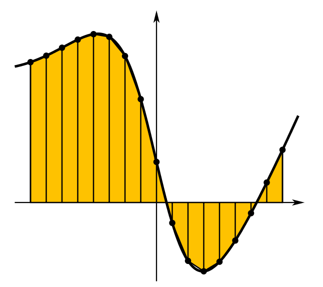
(Picture from Wikipedia)
The numerical integration code contained in RcppNumerical is based
on the NumericalIntegration
library developed by Sreekumar Thaithara Balan,
Mark Sauder, and Matt Beall.
To compute integration of a function, first define a functor inherited from
the Func class:
class Func
{
public:
    virtual double operator()(const double& x) const = 0;
    virtual void   operator()(double* x, const int n) const
    {
        for(int i = 0; i < n; i++)
            x[i] = this->operator()(x[i]);
    }
};
The first function evaluates one point at a time, and the second version overwrites each point in the array by the corresponding function values. Only the second function will be used by the integration code, but usually it is easier to implement the first one.
RcppNumerical provides a wrapper function for the NumericalIntegration
library with the following interface:
inline double integrate(
    const Func& f, const double& lower, const double& upper,
    double& err_est, int& err_code,
    const int subdiv = 100,
    const double& eps_abs = 1e-8, const double& eps_rel = 1e-6,
    const Integrator<double>::QuadratureRule rule = Integrator<double>::GaussKronrod41
)
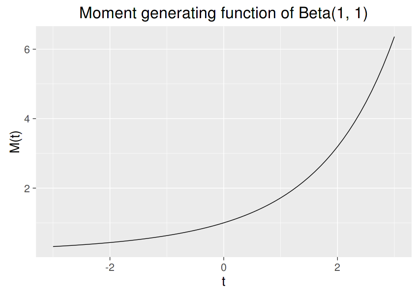
See the README page for the explanation of each argument. Below shows an example that calculates the moment generating function of a $Beta(a,b)$ distribution, $M(t) = E(e^{tX})$:
// [[Rcpp::depends(RcppEigen)]]
// [[Rcpp::depends(RcppNumerical)]]
#include <RcppNumerical.h>
using namespace Numer;

// M(t) = E(exp(t * X)) = int exp(t * x) * f(x) dx, f(x) is the p.d.f.
class Mintegrand: public Func
{
private:
    const double a;
    const double b;
    const double t;
public:
    Mintegrand(double a_, double b_, double t_) : a(a_), b(b_), t(t_) {}

    double operator()(const double& x) const
    {
        return std::exp(t * x) * R::dbeta(x, a, b, 0);
    }
};

// [[Rcpp::export]]
double beta_mgf(double t, double a, double b)
{
    Mintegrand f(a, b, t);
    double err_est;
    int err_code;
    return integrate(f, 0.0, 1.0, err_est, err_code);
}
We can compile and run this code in R and draw the graph:
library(Rcpp)
library(ggplot2)
sourceCpp("somefile.cpp")
t0 = seq(-3, 3, by = 0.1)
mt = sapply(t0, beta_mgf, a = 1, b = 1)
qplot(t0, mt, geom = "line", xlab = "t", ylab = "M(t)",
      main = "Moment generating function of Beta(1, 1)")

Numerical Optimization
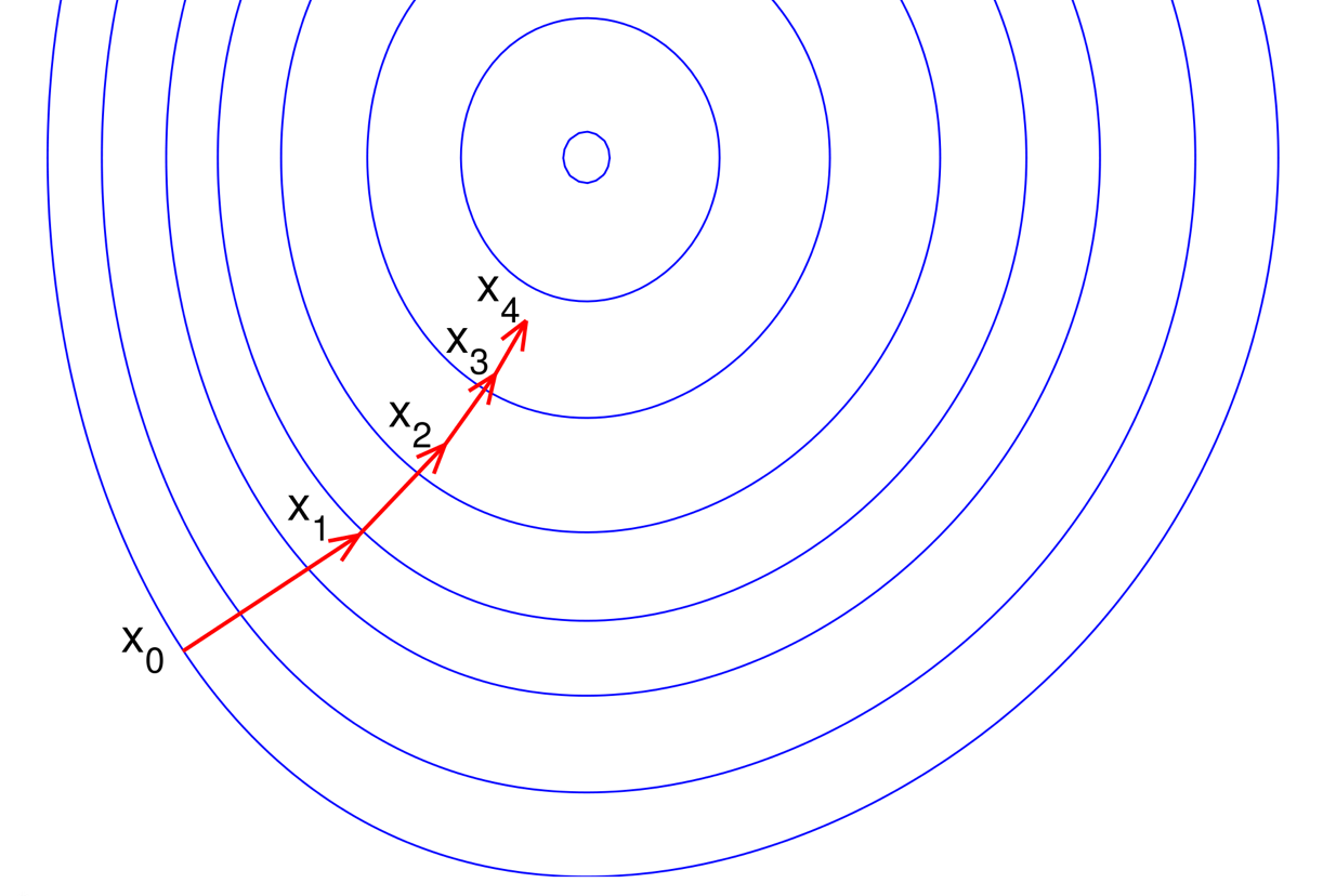
Currently RcppNumerical contains the L-BFGS algorithm for unconstrained
minimization problems based on the
libLBFGS library
developed by Naoaki Okazaki.

(Picture from aria42.com)
Again, one needs to first define a functor to represent the multivariate function to be minimized.
class MFuncGrad
{
public:
    virtual double f_grad(Constvec& x, Refvec grad) = 0;
};
Here Constvec represents a read-only vector and Refvec a writable
vector. Their definitions are
// Reference to a vector
typedef Eigen::Ref<Eigen::VectorXd>             Refvec;
typedef const Eigen::Ref<const Eigen::VectorXd> Constvec;
(Basically you can treat Refvec as a Eigen::VectorXd and
Constvec the const version. Using Eigen::Ref is mainly to avoid
memory copy. See the explanation
here.)
The f_grad() member function returns the function value on vector x,
and overwrites grad by the gradient.
The wrapper function for libLBFGS is
inline int optim_lbfgs(
    MFuncGrad& f, Refvec x, double& fx_opt,
    const int maxit = 300,
    const double& eps_f = 1e-6, const double& eps_g = 1e-5
)
Also refer to the README page for details and see the logistic regression example below.
Fast Logistic Regression: An Example
Let’s see a realistic example that uses the optimization library to fit a logistic regression.
Given a data matrix $X$ and a 0-1 valued vector $Y$, we want to find a coefficient vector $\beta$ such that the negative log-likelihood function is minimized:
$$\min_{\beta} -l(\beta)=\sum_{i=1}^n\left[ \log(1+\exp(x_i’\beta)) - y_i x_i’\beta\right]$$
The gradient function is
$$g(\beta)=X’(p(\beta)-Y),\quad p(\beta)=\frac{1}{1+\exp(-X\beta)}$$
So we can write the code as follows:
// [[Rcpp::depends(RcppEigen)]]
// [[Rcpp::depends(RcppNumerical)]]
#include <RcppNumerical.h>
using namespace Numer;
using Rcpp::NumericVector;
using Rcpp::NumericMatrix;
typedef Eigen::Map<Eigen::MatrixXd> MapMat;
typedef Eigen::Map<Eigen::VectorXd> MapVec;

class LogisticReg: public MFuncGrad
{
private:
    const MapMat X;
    const MapVec Y;
public:
    LogisticReg(const MapMat x_, const MapVec y_) : X(x_), Y(y_) {}

    double f_grad(Constvec& beta, Refvec grad)
    {
        // Negative log likelihood
        //   sum(log(1 + exp(X * beta))) - y' * X * beta

        Eigen::VectorXd xbeta = X * beta;
        const double yxbeta = Y.dot(xbeta);
        // X * beta => exp(X * beta)
        xbeta = xbeta.array().exp();
        const double f = (xbeta.array() + 1.0).log().sum() - yxbeta;

        // Gradient
        //   X' * (p - y), p = exp(X * beta) / (1 + exp(X * beta))

        // exp(X * beta) => p
        xbeta.array() /= (xbeta.array() + 1.0);
        grad.noalias() = X.transpose() * (xbeta - Y);

        return f;
    }
};

// [[Rcpp::export]]
NumericVector logistic_reg(NumericMatrix x, NumericVector y)
{
    const MapMat xx = Rcpp::as<MapMat>(x);
    const MapVec yy = Rcpp::as<MapVec>(y);
    // Negative log likelihood
    LogisticReg nll(xx, yy);
    // Initial guess
    Eigen::VectorXd beta(xx.cols());
    beta.setZero();

    double fopt;
    int status = optim_lbfgs(nll, beta, fopt);
    if(status < 0)
        Rcpp::stop("fail to converge");

    return Rcpp::wrap(beta);
}
Now let’s do a quick benchmark:
set.seed(123)
n = 5000
p = 100
x = matrix(rnorm(n * p), n)
beta = runif(p)
xb = c(x %*% beta)
p = exp(xb) / (1 + exp(xb))
y = rbinom(n, 1, p)

system.time(res1 <- glm.fit(x, y, family = binomial())$coefficients)
##  user  system elapsed
## 0.339   0.004   0.342
system.time(res2 <- logistic_reg(x, y))
##  user  system elapsed
##  0.01    0.00    0.01
max(abs(res1 - res2))
## [1] 1.977189e-07
This is not a fair comparison however, since glm.fit() will calculate some
other components besides $\beta$, and the precision of two methods are also
different.
RcppNumerical provides a function fastLR() that is a more stable
version of the code above (avoiding exp() overflow) and returns similar
components as glm.fit(). The performance is similar:
system.time(res3 <- fastLR(x, y)$coefficients)
##  user  system elapsed
##  0.01    0.00    0.01
max(abs(res1 - res3))
## [1] 1.977189e-07
Its source code can be found here.
Final Words
If you think this package may be helpful, feel free to leave comments or request features in the Github page. Contribution and pull requests would be great.
